Excel 2007
Knowledge for Physics
OpenOffice, a free alternative to Excel can be downloaded by click here or going to  .
.Objectives
- Learn how to use Microsoft Excel
- Learn how to insert data into a spreadsheet
- Learn how to format data and cells in Excel
- Learn how to sort data in Excel
- Learn how to do calculations in Excel
- Learn the difference between absolute and relative cell references
- Learn how to add rows and columns in Excel
- Learn how to insert text boxes in Excel
- Learn Learn how to create graphs in Excel
- Learn how to add and format trendlines in Excel
What is Microsoft Excel?
Microsoft Excel is a spreadsheet program which allows one to enter numerical values or data into the rows or columns of a spreadsheet, and to use these numerical entries for such things as calculations, graphs, and statistical analysis. Excel and other spreadsheet programs are used throughout the world in jobs, ranging from Accounting to Actuaries, from Insurance Agencies to Manufacturing industries, and in Academia and Science related fields like biology and physics.Vocabulary
- Absolute Reference – Absolute ranges have a $ character before the column portion of the reference and/or the row portion of the reference. The $ character indicates to Excel that it should not increment the column and/or row reference as you fill a range with a formula or as you copy a range. If you enter =A1 in a cell and then fill that cell down a column, the '1' in the reference will increment in each row. Thus, the formula in row 50 would be =A50. However, if you enter =$A$1 in a cell and fill down, the range reference will remain $A$1 -- it will not increment as you fill or copy down a column.
- Automatic Cell Filling – The ability to fill out some cells with values that belong to a common series.
- Cell – the small boxes where data exists in a spreadsheet
- Column – Cells that are in a vertical line of each other
- Function – just like in math, an
operation
performed on variables or constants
- Rows
– Cells that are in a horizontal line of each other
The Assignment
Your assignment is to complete all of the steps below and submit to your course instructor all of the pages that you are asked to print in the document below. These pages should be submitted in the order they appear, and should be stapled together.EXCEL
- Start Excel.
- Find Excel in your program menu and select it.
- Once the program loads a screen should appears that looks like the one below.
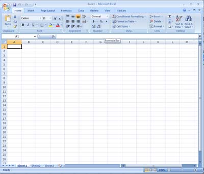
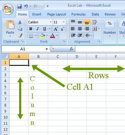
The first column in the spreadsheet is labeled A, and the first row is labeled 1. Spreadsheets use a coordinate system to access information. Each cell in the spreadsheet is identified by the letter-number combination of its location. Therefore you have cells names A1, B1, B2, B3, and so on.
Inserting Data
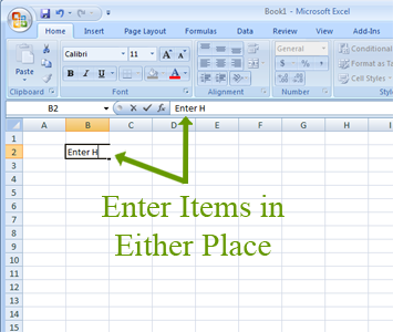
- To insert data into excel select the cell in which you would like to enter the data.
- At this point you can enter the data in 1 of 2 spots
- Primarily you will enter the data directly into the cell.
- In some cased you will enter data into the formula bar.
At this point lets practice entering some data: Please make a table as it is described below.
- Enter in cell A1 "Data"
- Enter in cell A2 "Car Number -"
- Enter in cell A3 "Track Number -"
- Enter in cell A4 "Mass (kg)="
- Enter in cell A6 "Trial"
- Enter in cell B6 "Distance (m)"
- Enter in cell C6 "Time (s)"
- Enter in cell D6 "Acceleration (m/s2)"
- Enter in cell E6 "Force (kg m/s2)"
- Enter in cell B2 "4"
- Enter in cell B3 "2"
- Enter in cell B4 "3"
- Enter in cell A7 "1"
- Enter in cell A8 "2"
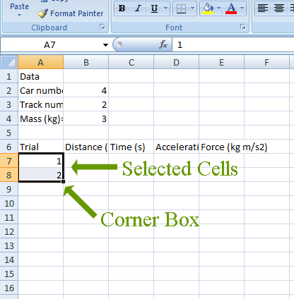
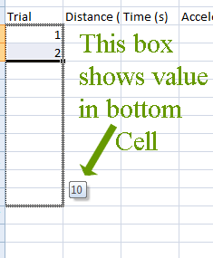
- Select cells A7 and A8 by highlighting them.
- Click on the small box in lower left hand corner of the selected cells and drag it down to 10. This is called Automatic Cell Filling
- Enter the following distances for trials 1-10
- 9.95
- 10.03
- 10
- 9.9
- 10.1
- 10.08
- 10.03
- 9.98
- 10.03
- 9.99
- Enter 10 random times for trials 1-10 that are between 1.05 and 1.95 seconds.
- You chose a value between 1.05 and 1.95
- You chose a value between 1.05 and 1.95
- You chose a value between 1.05 and 1.95
- You chose a value between 1.05 and 1.95
- You chose a value between 1.05 and 1.95
- You chose a value between 1.05 and 1.95
- You chose a value between 1.05 and 1.95
- You chose a value between 1.05 and 1.95
- You chose a value between 1.05 and 1.95
- You chose a value between 1.05 and 1.95
- Save your document naming it "LastName_Excel_Lab"
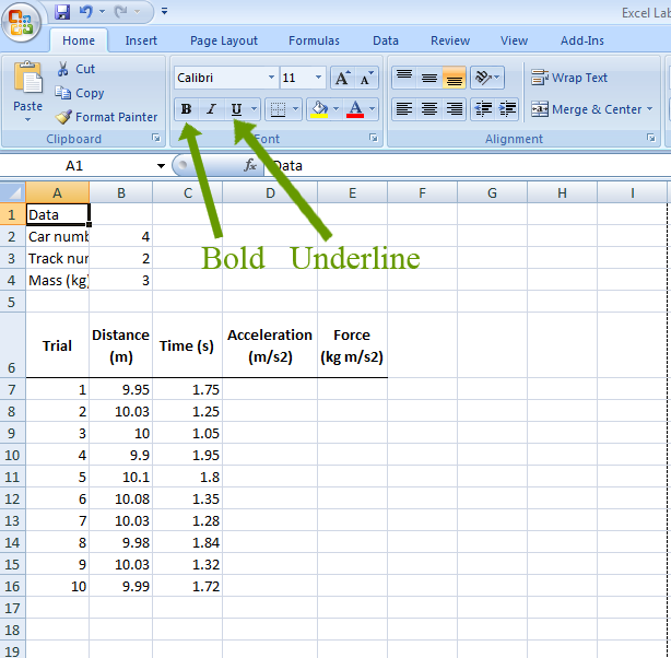
Formatting
- Select boxes A6 through E6
- Right click on the selected boxes and choose Format Cells.
- Chose the alignment tab
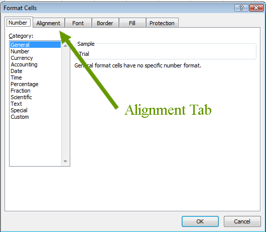
- Under Text Alignment choose Horizontal: Center.
- Under Text control choose wrap text.
- Choose the font tab
- Under Font Style chose bold
- Choose the boarder tab
- Select a lower boarder only
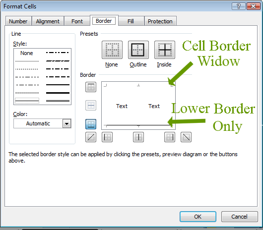
- Press OK
- At this point you should notice that the distance, acceleration, and force cells need to be resized.
- Click at the top of the column window between B and C you can changed the width of the column so that Distance is on the first line and (m) is on the second.
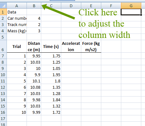
- Adjust the column with for acceleration too
- For Force cell put to extra spaces after the word Force.
- Click on cell A1
- Select bold and underline from the home menu
- At this point, realizing adjusting column A would make it out of proportion with the table so we will need to move the data from column B to the right and merge certain cells.
- Now select B2, B3, and B4
- Use the cut function
- Click on C2 and paste the data
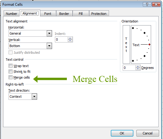
- Select A2 and B2
- Right click on the selected cells
- Choose format cells
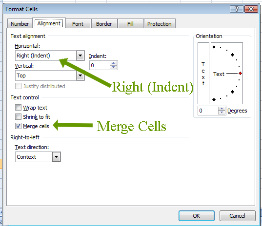
- Click on the Alignment Tab
- Under Text Controls click Merge cells.
- Press OK
- Select A3 and B3
- Right click on the selected cells
- Choose format cells
- Click on the Alignment Tab
- Under Text Controls click Merge cells.
- Press OK
- Select A4 and B4
- Right click on the selected cells
- Choose format cells
- Click on the Alignment Tab
- Under Text Controls click Merge cells.
- Press OK
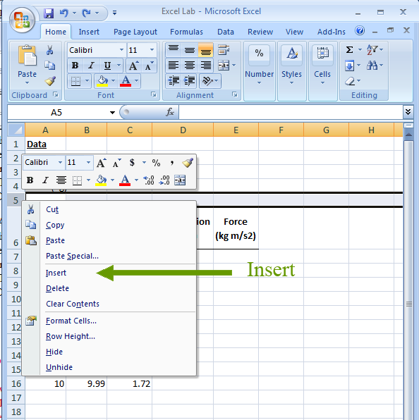
- Realizing at this point that we have never accounted for the initial position, we need to add the data below the mass line.
- Right click on the "5" of row 5
- Select insert
- Merge cell A5 and B5
- In A5 type "Initial Velocity (m/s) -"
- Expand column B to make everything in the step above fit into A5 and B5
- In C5 enter "0"
- For acceleration and force we need to make the 2's an exponent.
- Click on D7
- In the formula bar select the "2"
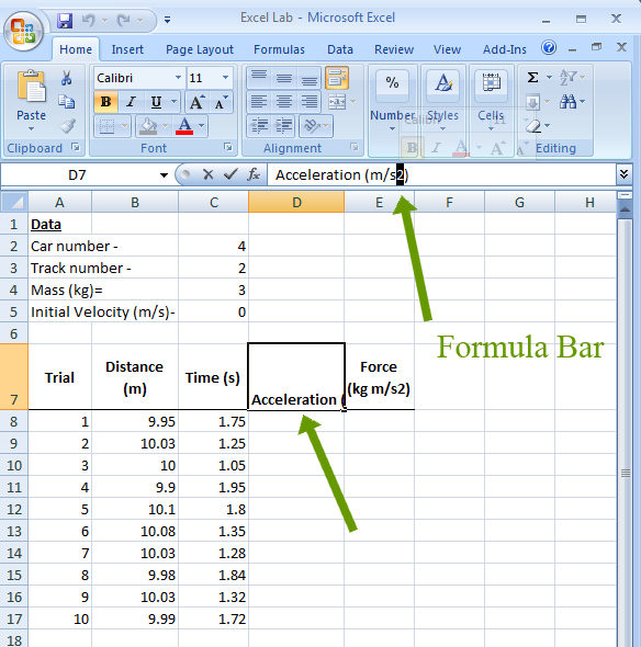
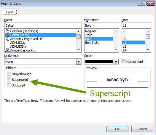
- Expand the font menu
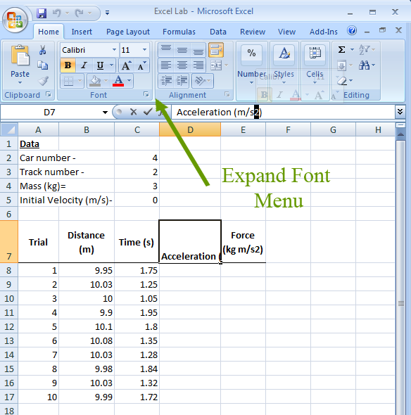
- In this menu, under effects, choose Superscript.
- Repeat this process to superscript the 2 in cell E7,
- There is also a need to standardize the decimal value of the cells associated with these calculations.
- Chose cells B8 through E17.
- Right click in the selected cells.
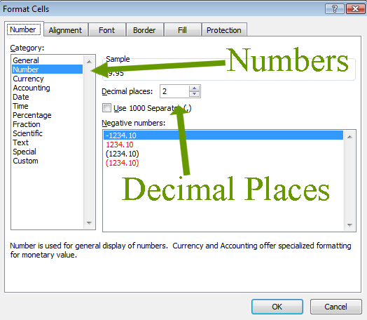
- Choose format
- Select the number tab.
- Under "Category" choose "Number"
- In the middle of this widow make sure the decimal places are marked "2"
- Click OK
- SAVE YOUR WORK
Calculations
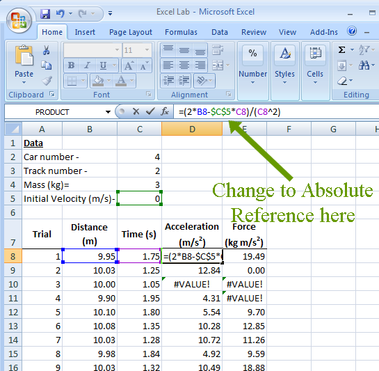
- We are going to calculate the acceleration using the equation a=(2d-vo*t)/(t2)
- Click in box D8
- Type "="
- Type "("
- Type "2"
- Type "*"
- Click on cell B8
- Type "-"
- Click on cell C5
- Type "*":
- Click on cell C8
- Type ")"
- Type "/"
- Type "("
- Click on cell C8
- Type "^"
- Type "2"
- Type ")"
- Type enter
- Now we are going to calculate force (F=m*a) in cell E8.
- Click on E8
- Type "=" (Note: every formula starts with an equals sign)
- Click on Cell C4 (Note: Here you are calling the value from cell D8)
- Type "*"
- Click on cell D8
- Type enter
- select D8 and E8 and perform an automatic cell fill down to row 17 by clicking in the lower right hand corner of the selected window and dragging selection box down.
- At this point you should notice there are some errors.

These errors are caused because when we auto fill, it adjust the cell values in the formula to match the reference location for each row. For example what was called B8 in row 8 would be called B9 in row 9 or B10 in row 10. This is good because it uses the data on the left to calculate the values on the right. But this becomes bad when you have a parked piece of data like the mass and the initial velocity. You have 2 options here. The first is to make another column and repeat the same mass in each row. This looks messy and shouldn't be done for professional work. Option 2 is to make an absolute reference which will make the called value not increment when you auto fill. There are 3 reference styles which are listed below.
| $A$1 | Both
the column and row reference are fixed. Neither will be incremented or
changed during a copy or fill operation. |
| $A1 | Only the column reference is fixed.
It will not change during a fill or copy, but the row will change. |
| A$1 | Only the row reference is fixed. It will not change during a fill or copy, but the column will change. |
The way we are going to do this is as follows
- Click on cell D8
- In the formula bar change C5 to $C$5
- Press Enter
- Now auto fill the acceleration calculations again.
- Note: The force values changed when you changes the Acceleration column
- Click on cell E8
- Make C4 Absolute by changing it to $C$4
- Press Enter
- Auto fill the Force calculations.
Now you want to calculate the average of a row and also calculate percent error. This will allow us to see how to call some built in functions of the program.
- Enter into cell A18 "Average="
- You may need to adjust the width of column A slightly to make it fit
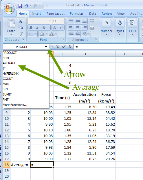
- In B18 type "="
- To the left of the formula bar a drop down menu will now appear.
- Select Average in this menu.
- A box should now appear.
- In this box there are 2 cells listed next to "Number1." These cells probably B8:B17. This is read B8 to B17. The average function will then take the average of the numbers between these 2 cells.
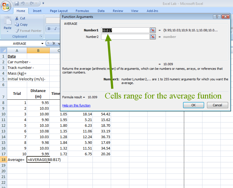
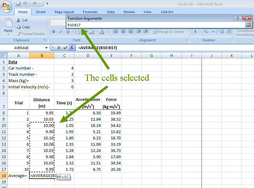
Note: if you want to change this range you may type in the cell range or you may click and drag across the cells you want to use to select the cells.
- Make sure you are taking the average of B8:B17 and then press "OK"
- Now auto fill B18 to the right getting the average of Time, Acceleration and Force.
- Select Cells A18 through E18
- Format the cells using the properties, boarder tab and adding a top boarder only.
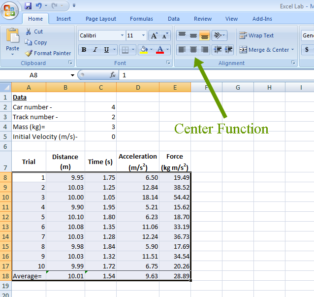
- Select cells A8 to E18
- Press the center function in the alignment box of the home tab
- Click on cell A18 and bold face the text in this box.
- Select cells B18 through E18
- Right click and select format cell
- Click on the the Number tab
- Under categories make sure "number" is selected
- Change the decimal places to 1. We need to do this because when we look back at our original distance data, there were some measurements only read to the tenth spot. We need to accurately portray the averages with the correct number of significant figures.
- Select cells C2 through C5 and left justify them with the function button in the alignment box of the home tab.
- In cell A20 type "Theoretical Acceleration="
- In cell A21 type "Experimental Acceleration="
- In cell A22 type "Percent Error="
- Select Cells A20 through C20
- Right click and choose format cell
- In the Alignment tab select merge cells
- Also in the Alignment tab, under text alignment, choose Horizontal Right (Indent)
- Select Cells A21 through C21
- Right click and choose format cell
- In the Text alignment tab select merge cells
- Also in the Alignment tab, under text alignment, choose horizontal right (indent)
- Select Cells A22 through C22
- Right click and choose format cell
- In the Alignment tab select merge cells
- Also in the Alignment tab, under text alignment, choose horizontal right (indent)
- Type in D20 "9.8" and press enter
- In D21 Type "=" then select D18 and press enter
- Now we are going to calculate the percent error which is equal to |(theoretical-experimental)/theoretical)|*100%
- In D22 type "="
- Then from the function drop down bar next to the formula bar select "More Functions..."
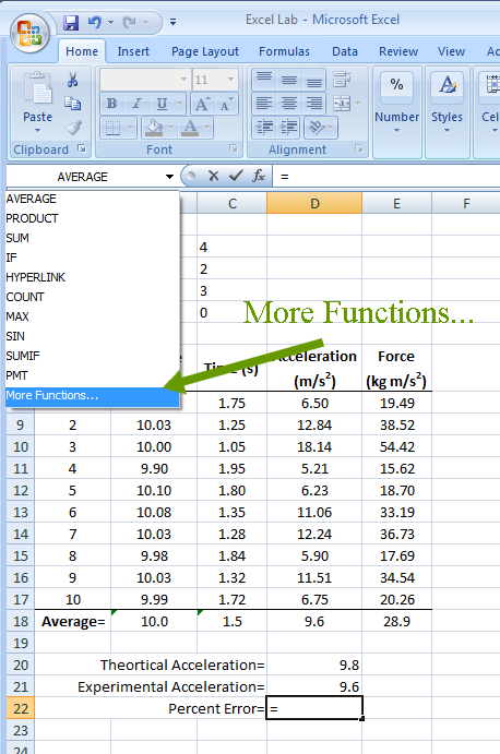
- In this more function widow you can see that excel has a wide variety of functions ranging from taking the squre root, to suming a set of data, trignotetic functions. The function we want to use now is the absolute value function.
- Choose all from the catagory window
- Then select ABS and press ok
- You could have also searched for the function.
- In the function window that now appears type the following "("
- Now click D20
- Type "-"
- Click D21
- Type ")"
- Type "/"
- Click D20
- Your fomula should look like the box below.
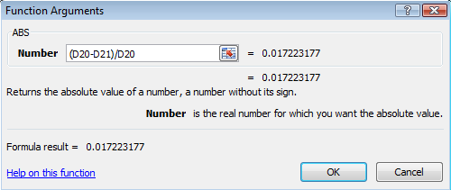
- click ok
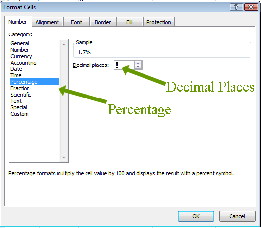
- Right click on D22
- Select Format Cell
- Click on the Number tab
- Under catagory choose percentage
- For the decimal places again choose 1
- Click ok
- Choose A20 through A22
- Select Bold from the font box of the home bar.
- In E20 type m/s2
- In E21 type m/s2
- Format E20 and E21 super script the 2 to make it look lik m/s2
- SAVE YOUR WORK
Graphing Data
Graphing data is important because it allows us to visualize the relationship between the data and calculated values.We are now going to graph Force vs Acceleration
- Select cells D8 through E17
- Select the insert tab from the top of the excel window
- In the chart box click on Scatter
- Choose Scater with Markers Only
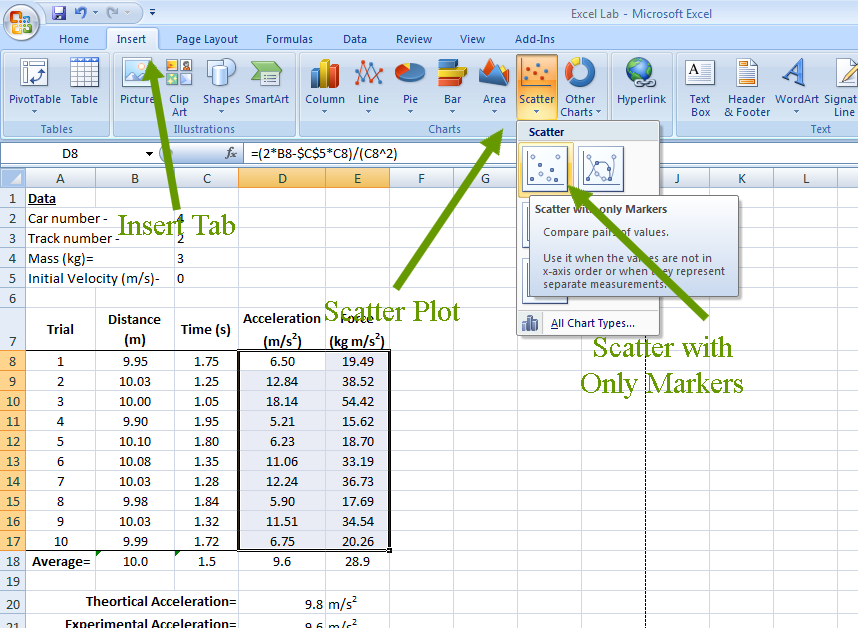
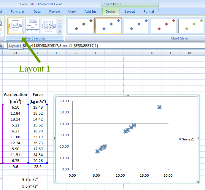
- A chart should appear
- In the design tab under chart layout
- Choose layout 1
- In the graph double click on chart title and change it to "Force vs Acceleration"
- Double click on the x axis title and change it to "Acceleration (m/s2) Note: To superscript the 2 you need to click on the home tab of the main menu and then expand the Font Box so that you can check the superscript box.
- Double click on the y axis title and chang it to "Force (kg m/s2) Note: Again superscript the 2.
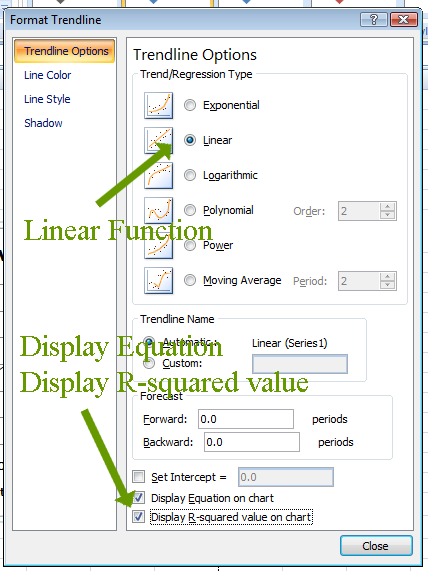
- Add a trendline by right clicking on one of the data points and choosing "Add Trendline"
- In the add trandline window
- Click on the trendline equation text box and move it to the upper right hand corner of the graph window.
- Right click on the legend on the right hand side of the graph and select delete.
- Right click on one of the x axis values and then select "Add Major Gridlines"
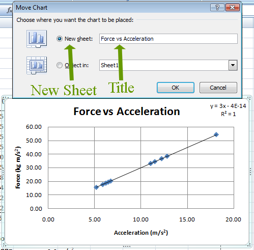
- If you wanted to paste this into a word document you could copy and past the graph from here to the word document. If you are going to print the graph as its own page (which you are doing for this assignment) do the following :
- Right click in the lower left hand corner and select "Move Chart...
- Select "New Sheet
- Title it "Force vs Acceleration"
- Click OK
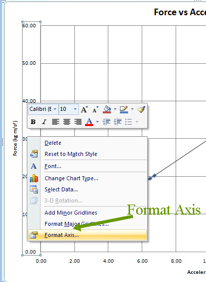
- In the new window, right click on the "y-axis"
- Choose format axis
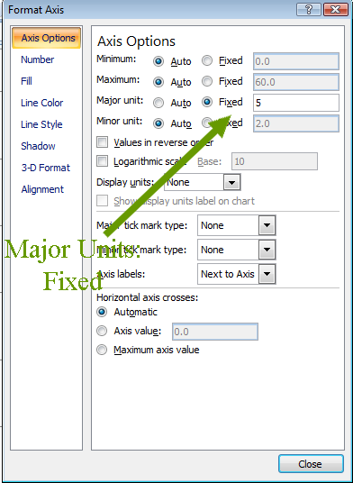
- Under Axis Options
- Change Major units to fixed
- Change the value to 5
- Click close
- Right click on sheet tab 2 and select delete
- Right click on sheet tab 3 and select delete
- Right click on sheet tab 1 and select rename
- Type "Data"
- Select the Data Tab
We will now make an inverse square graph.
- Select C8 through D17
- Insert a Scatter With Only Marks Graph
- Title this Acceleration vs Time
- Label the x-axis as Time (s)
- Label the y-axis as Acceleration (m/s2)
- Delete the Legend
- Right click on a Data Point
- Add trendline
- Chose a power function under regression type
- Diplay Equation
- Display R-squared
- Move the equation box to the upper right hand corner.
- Move the graph to a new sheet
- Name it : Acceleration vs Time
- Right click on an x-axis unit
- Add major gridlines
- Right click on an x-axis unit again
- Select Format Axis
- Change the major axis to fixed with 0.1 increments
- Right click on the a y-axis unit again
- Select Format Axis
- Change the major axis to fixed with 1.0 increments
- SAVE YOUR WORK
Sort
- Click on the Data tab
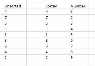
- In cell B25 type "Unsorted"
- In cell D25 type "Sorted"
- In cell E25 type "Number"
- Bold and Underline the the words in cell B25, D25, and E25
- Enter the data found in the image below
- Select B25 through E34
- Center information
- Select cells D26 through D34
- Select the Data Tab
- In the Sort & Filter Box select Sort A to Z
- Expand the selection to include E26 through E34
- Click Sort
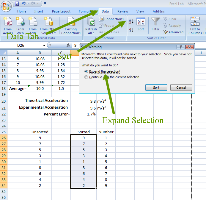
Note the data in the sorted column is now in order, while the data in the number column still matches up with the value it was next to in the unsorted chart.
- SAVE YOUR WORK
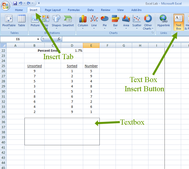
Text Boxes
Text boxes are a way to add text to a spreadsheet that is not bound by the cells.- Click on the insert tab
- Then in the text box click text box
- Your cursore will not point into a vertical arrow pointed down.
- Click at the upper corner of B36 and drag to E40
- By left clicking on the left corner of the newly formed text box you will see a blinking curser
- You can now type just like you were in a word processing program.
- Type in this box "This data is used to show how to sort data."
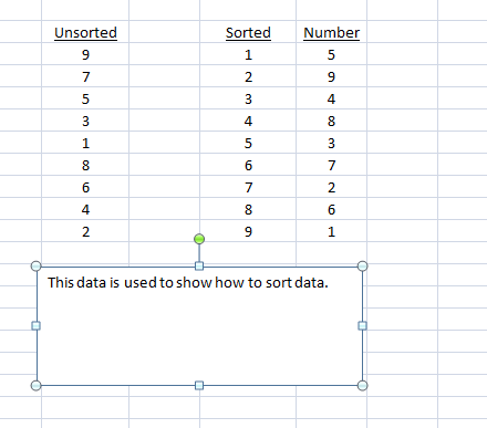
- You can now click on the lower right hand corner of the textbox and shrink it to the lower corner of C39
- You can now pick up the textbox and drag it so the upper left had corner is located at the top left hand corner of G29
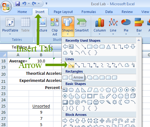
- Click the Insert Tab
- Click Shapes
- Chose the arrow under lines shape
- Click at the left sizeing box of the textbox
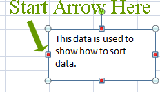
- Drag the arrow so the head is at the top left hand corner of F30
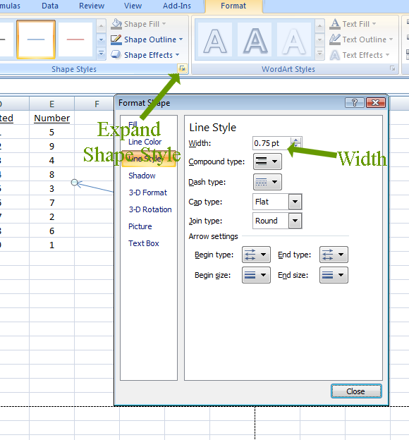
- Click on the arrow
- In the Format Tab click and expand the Shape Style box
- Under Line Styles increase the width to 3
- SAVE YOUR WORK
Finalizing your Document
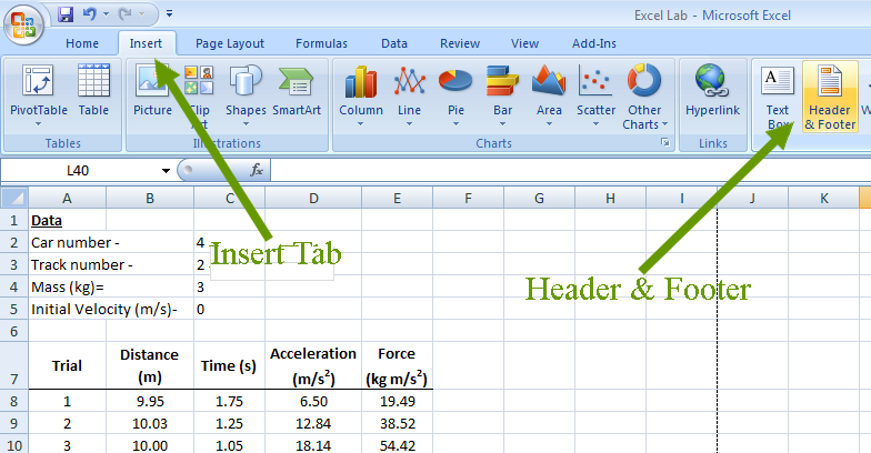
We need to insert a header and a footer.
- Click on Insert Tab
- Click on Header and Footer in the Text Box
- In the left hand Header Box Type your name
- Press return
- Type "Mr. Croom's Physics"
- In the right box type today's date
- Press return
- Type "Excel Lab"
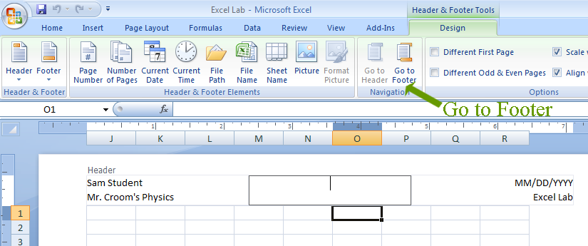
- Click the "Go to Footer" button
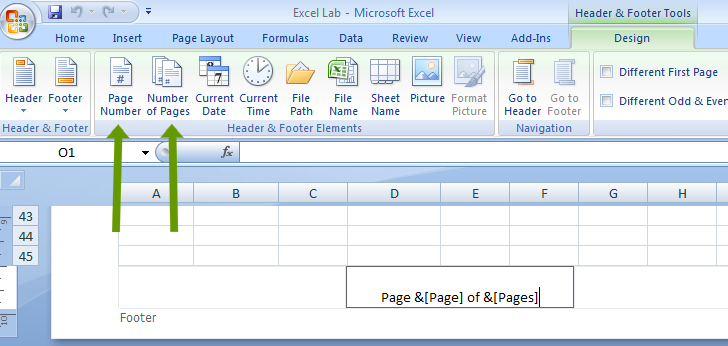
- In the center footer box type "Page " Note: there is a space after "Page"
- Click "Page Number"
- Type " of " Note: there are spaces before and after "of"
- Click "Number of Page"
- Click somewhere else on the screen
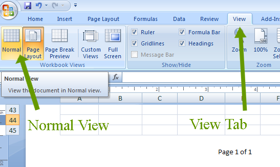
- Click the View Tab
- In the Workbook Views Box Click Normal View
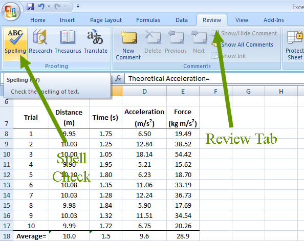
Now we need to run Spell Check
- Click on the review tab
- In the Proofing Box click Spelling
- SAVE YOUR WORK
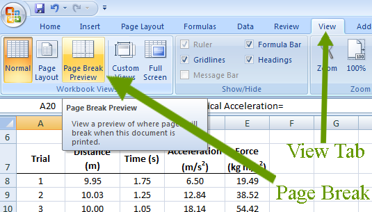
- Click the View Tab
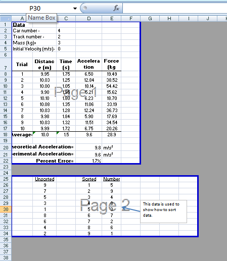
- In the Workbook Views Box click "Page Break Preview"
- Select cells A1 through F22
- Right click on the area and choose "Set Print Area"
- Select cells A25 through I34
- Rick click on the area and choose "Add to Print Area"
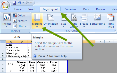
- Click on the page Layout Tab
- In the Page Setup box click on "Margins"
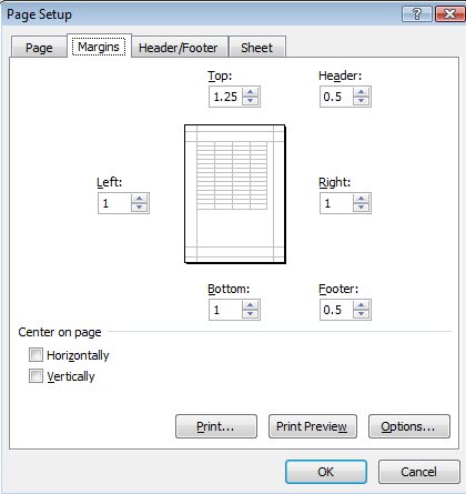
- Then click "Custom Margins"
- Set the Top Margin to 1.25
- Set the Left Margin to 1
- Set the Right Margin to 1
- Set the Bottom Margin to 1
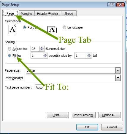
- Click the Page Tab
- Under Scaling Select Fit to
- Set the values to 1 page wide by 1 page high
- Click OK
- SAVE YOUR WORK
- Print a pdf of the entire workbook
- Follow the directions found at http://www.wikihow.com/Convert-Excel-to-PDF to determine how to print the workbook to a PDF.
- Make sure your PDF has the following pages.
- Page 1
- Page 2
- Force vs Acceleration
- Acceleration vs Time.
- Upload your PDF document to TurnItIn
CONGRATULATIONS! You have Finished the Physics Excel Tutorial